In this walkthrough, we will simulate and design a basic microfluidic system, a single Taylor Cone emitter atop a cylindrical channel. We will choose the propellant, set the geometry, then plot thrust and specific impulse (Isp) against extraction voltage. Components will be designed using the Domain Modeler and flow simulation will occur in the freely-available, 3rd-party LTSPICE tool.

1. Go to the Domain Modeler. If you are redirected to the login screen, enter your credentials. This will begin a 3-hour session.

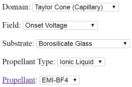
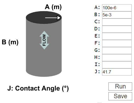
2. First, we will create a capillary Taylor cone. In the Domain Modeler, make the following selections from the pull-down menus, then press the Run button:

3. In the metadata textarea there will be a value for every field option, and an explanation of how those values were calculated. The chart will be specific to the currently selected field, onset voltage. Hover your mouse over the chart to see the precise value.

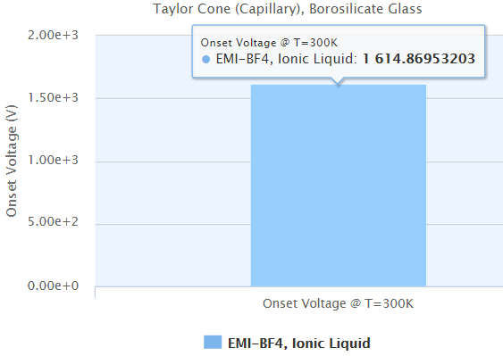
4. Suppose that we would like to reduce the onset voltage. In the metadata textarea we can see that onset voltage scales with the square root of surface tension (see excerpt, below). Let's use the Propellant Database to find a propellant with a lower surface tension. Click the Propellant link on the left side of the screen to open the Propellant Database in a new tab.

"... Onset Voltage: 1.61487e+03 V
sqrt(γ*Rc/ε0)*ln(β*s/Rc), where γ is the surface tension, Rc is the capillary radius, ε0 is the permittivity of free space, β is an empirical parameter between ~2 and 4 and s is the spacing between the tip of the cone and the extractor electrodes. The expression is derived from the assumption that once the electric force exceeds the balance between the surface tension force or pressure (2*γ/Rc) associated with the convex meniscus protruding from the capillary and the electric field force (0.5*ε0*E^2) to pull the liquid into the meniscus, a Taylor cone will form. The ln factor is derived from a hyperboloid model of the tip which allows an analytical solution of the Laplace equation (which then gives β=4). Reference: Courtney, D. G., H. Q. Li, and P. Lozano (2012), "Emission measurements from planar arrays of porous ionic liquid ion sources", J. of Phys. D: Appl. Phys., 45, 48, 485203. ..."

5. Select Surface Tension from the Field pulldown menu, set Tmin and Tmax both equal to 300, then press Submit (or Enter).

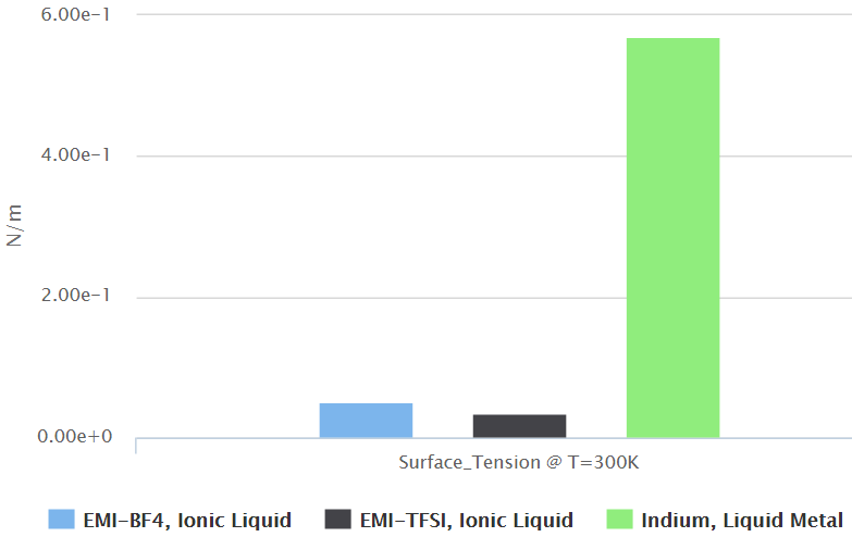
6. Remove Indium from the chart to better visualize the difference between EMI-BF4 and EMI-TFSI. Do this by clicking "Indium, Liquid Metal" in the legend. When this happens, the chart autoscales to clearly show that the surface tension of EMI-TFSI is about 30% less than EMI-BF4.

7. Go back to the Domain Modeler and change the propellant to EMI-TFSI, then press the Run button to see the new onset voltage. Take note of this value. Save this component to your user session by pressing the Save button.

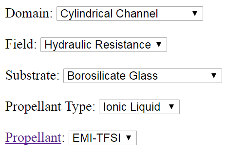
8. Now we will create a cylindrical channel with the same propellant and substrate as the Taylor Cone. Make selections in the Domain Modeler pull-down menus as shown below, then press Run. Then, set the cylinder radius to 10um in Box A (to match the Taylor Cone radius) and press Run.

9. A bar chart will appear at the bottom of the screen, displaying the hydraulic resistance. Suppose that we would like to reduce this resistance. The metadata textarea tells us that resistance scales with channel length. Change the cylinder height from 10mm to 5mm in Box B and press Run to see how the resistance changes.

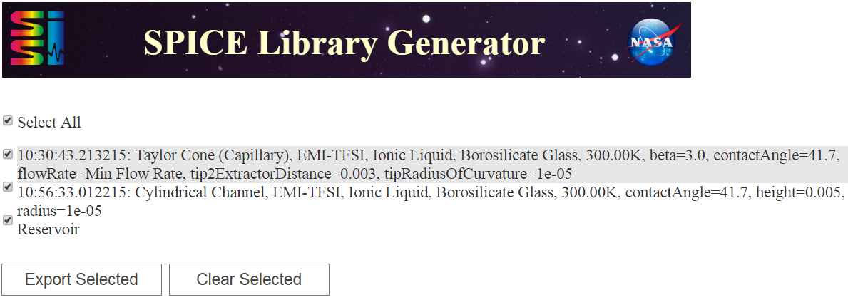
10. Save this component to your session by pressing the Save button. Now we are ready to download our saved components. Click on the "Export Saved Components" link on the bottom right corner of the Domain Modeler to open the Spice Library Generator page. Select all of the components and press the "Export Selected" button. This will download a zipped directory. Navigate to this directory on your local computer and unzip it.

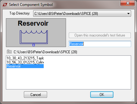
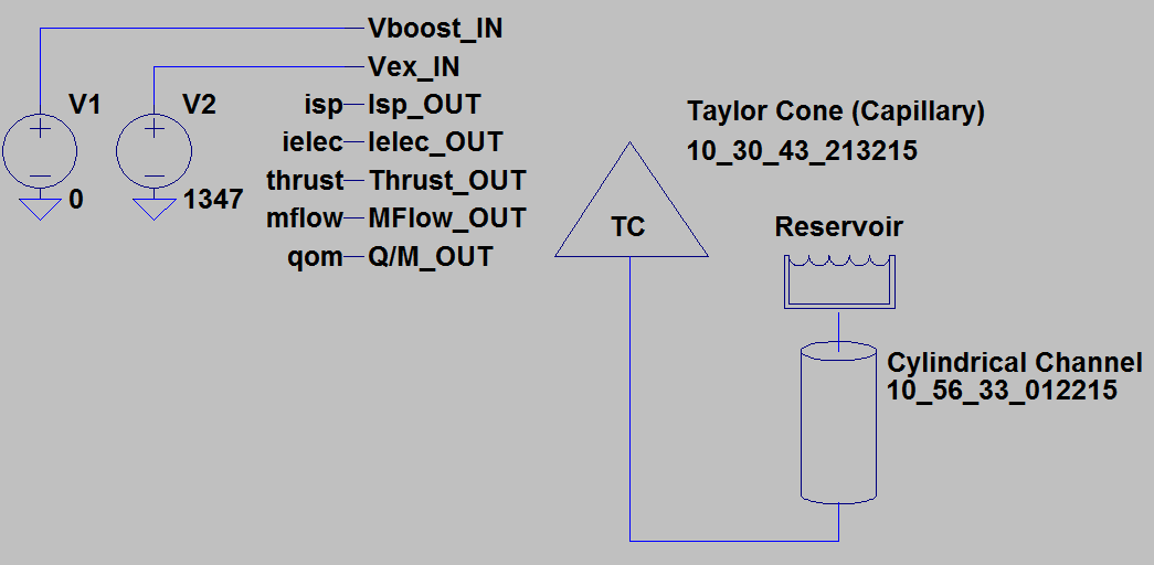
11. Download and install LTSPICE if you have not already done so. LTSPICE is a lightweight (< 40MB download) electrical circuit simulator. Open LTSPICE and create a new schematic (File --> New Schematic). Save this schematic to the same directory as your downloaded components (File --> Save As). Bring up the "Select Component Symbol" window (Edit --> Component) and choose your unzipped component directory from the "Top Directory" pulldown menu. Place the cylindrical channel, Taylor Cone and reservoir components on the schematic as shown below (in Step 12). Connect them together with wires (Edit --> Draw Wire).

12. The Taylor Cone has two inputs, the extraction voltage (Vex_IN) and the booster grid potential (Vboost_IN). To set these inputs, we will put two voltage sources on the schematic as shown below. Bring up the "Select Component Symbol" window and navigate to the default LTSPICE component directory (e.g. LTSPICE\lib\sym) in the "Top Directory" pulldown. Select the "voltage" component and drop two of them on the schematic. Connect two ground terminal components (Edit --> Place GND) to the negative terminals of the voltage sources and wire the positive terminals to the Taylor Cone inputs. Right-click on the voltage source that is connected to Vboost_IN and set its value to zero. Right-click on the voltage source that is connected to Vex_IN and set it to a value slightly higher than the onset voltage. Finally, place unique labels on each of the Taylor Cone outputs (Edit --> Label NET). These labels will help you to find the desired information in the simulation result.

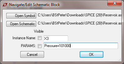
13. Right-click on the reservoir component and set the pressure to 101,000 Pa (~1 atm).

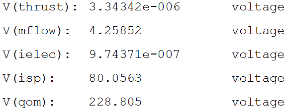
14. Open the "Edit Simulation Command" window (Simulate --> Run). Select the "DC Op Pnt" tab and press OK. This will produce a text-based result with many lines of diagnostic information. The most important lines are shown below. These values are reported as voltages, but should be interpreted as having the same units as in the Domain Modeler.

15. After having run a simulation, you can read the voltage at various points in the circuit by hovering or clicking your mouse on the wires. Except when dealing with the Taylor Cone input and output parameters, these voltages should be interpreted as pressures (Pa). The current, which can be interpreted as fluid flow (μL/s), can be read by clicking or hovering over the component nodes.

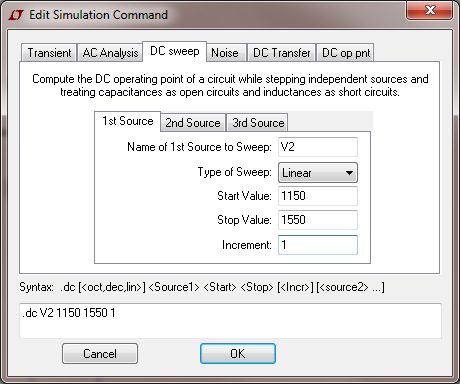
16. We will now plot thrust and Isp as a function of extraction voltage. Delete the ".op" line from your schematic (Edit --> Delete), then open the Edit Simulation Command window. In the "DC Sweep" tab, identify the name of the source to be swept (V2 in this example), the start and stop values, and an increment. Choose a range that goes both below and above the onset voltage.

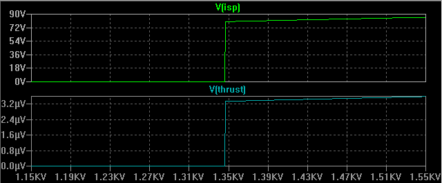
17. A blank chart will appear. Right-click and select "Add Plot Pane". In the top pane, right-click and select "Add Trace", then choose "V(isp)". Next, add "V(thrust)" to the bottom pane.

Congratulations, you've just simulated your first microfluidic circuit in the ESPET environment!